PROGRAMMING SYNTHESIZERS
The Synthesizers Playground
Jupylet includes a flexible and novel sound synthesis framework with which you can create subtractive, additive, frequency modulation, and sample based sound synthesizers, as wild as you can dream up.
It includes the following building blocks, all of which are implemented in pure Python and Numpy, the Python scientific computing library, for you to play with:
Continuous colored noise generators.
Antialiased wave oscillators with frequency modulation.
Resonant digital filters with sweepable cutoff frequency.
Multisampled instruments with frequency modulation.
ADSR envelopes with linear and non-linear curves.
Schroeder type algorithmic reverbs.
Convolution reberb.
Phase modulator.
Overdrive.
A sound synthesizer is in essense an audio signal processing graph. Audio signals are manipulated and transformed as they travel through the signal processing graph from its input to its output.
More generally, since each transformation applied to the audio signal is a computation, a software sound synthesizer is a computational graph.
In recent years there has been an explosion of tools and frameworks to represent and work with a different kind of computational graph that is rapidly growing in popularity and importance - the artificial neural network.
One of the most successful and surely the most Pythonic of them all is the wonderful Pytorch. Jupylet borrows from Pytorch the natural way in which it represents computational graphs.
Oscillators
Let’s start with a simple sawtooth Oscillator:
osc = Oscillator('sawtooth')
In Jupylet, all audio elements from basic building blocks to compound
synthesizers are Sound instances, the parallel
of a Pytorch nn.Module, and similarly you typically apply them to an input
to produce an output.
Let’s apply the oscilator to generate 44100 frames which is the default number of samples per second used by Jupylet and the sampling rate most commonly used in recorded audio:
In []: a0 = osc(frames=44100)
In []: a0
Out[]: array([[-0.07100377],
              [-0.05801778],
              [-0.04733572],
              ...,
              [-0.86131287],
              [-0.81941793],
              [-0.83591645]])
These numbers are time series values corresponding to a sawtooth signal. Let’s visualize them by plotting the first 169 numbers:
get_plot(a0[:169])
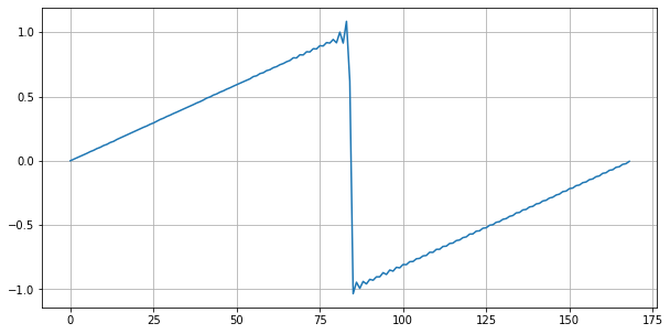
The little waves on the sawtooth are actually a good thing. This is how an anti-aliased sawtooth wave should look like.
You can play this array to hear how it sounds with:
sd.play(a0)
In Jupylet you can use an audio signal to modulate the frequency of an oscillator; it is called frequency modulation (FM). Let’s use a 100Hz sine wave to modulate the frequency of a 1000Hz sine wave:
osc0 = Oscillator('sine', 100)
osc1 = Oscillator('sine', 1000)

a0 = osc0() * 12
a1 = osc1(a0)
Frequency modulation is done in logarithmic scale with semitones as units; in this case we multiply the modulating signal by 12 so the carrier signal is modulated by one octave (12 semitones) up and down. Let’s see how the signal looks like:
get_plot(a1)
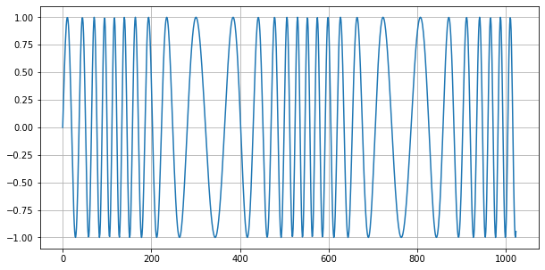
Note
The units on the x axis are frames or samples; therefore, at a sampling rate of 44100Hz the 1024 samples shown in the plot correspond to approximately 23ms.
A Simple Synthesizer
We can now take these two oscillators and write our first simple FM synthesizer:
class SimpleFMSynth(Sound):

    def __init__(self):

        super().__init__()

        self.osc0 = Oscillator('sine', 10)
        self.osc1 = Oscillator('sine')

    def forward(self):

        a0 = self.osc0() * 12
        a1 = self.osc1(a0, freq=self.freq)

        return a1
Let’s instantiate it and play a few notes, and while we’re at it, let’s also learn how to grab a recording of the audio output:
synth = SimpleFMSynth()

start_recording()

synth.play(C6)
await sleep(1/2)

synth.play_release()
await sleep(1/2)

synth.play(D6)
await sleep(1/2)

synth.play_release()
await sleep(1/2)

synth.play(E6)
await sleep(1/2)

synth.play_release()
await sleep(1/2)

a0 = stop_recording()
sf.write('simple-fm-synth.ogg', a0, 44100)
Gates and Envelopes
Traditonally, analog synthesizers consist of electronic circuits that generate, transform, and combine audio signals. Starting in the 70s synthesizers have begun using electric signals called control voltage and gates, or CV/gate for short, to control the pitch, onset, and duration of the generated audio signals.
You can visualize a gate as an electric voltage that is generated by pressing a keyboard key to control the flow of other audio signals (e.g. a sine wave) through the circuitry, just as a physical gate would control the flow of people in the street.
While these signals are not strictly necessary today they are still sometimes used in modern equipment, and in particular Jupylet makes use of a gate construct to control the precise timing of the onset and duration of sounds.
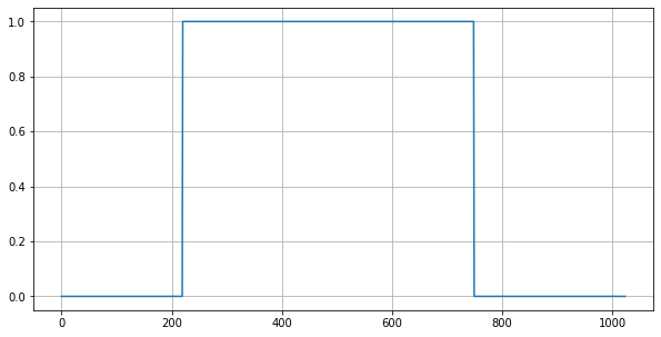
The concept of a synthesizer gate fits elegantly into the conception of a synthesizer as a computational graph, as a simple multiplcation operation. Let’s see it in action:
gate = LatencyGate()

gate.open(dt=0.005)
gate.close(dt=0.012)

g0 = gate()
get_plot(g0)
The GatedSound class employs a
LatencyGate to implement precise onset
and duration of notes. Let’s see how to use it to improve our simple
synthesizer:
class SimpleFMSynth2(GatedSound):

    def __init__(self):

        super().__init__()

        self.osc0 = Oscillator('sine', 10)
        self.osc1 = Oscillator('sine')

    def forward(self):

        g0 = self.gate()

        a0 = self.osc0() * 12
        a1 = self.osc1(a0, freq=self.freq)

        return a1 * g0
And now we can simplify the code that generates our three little notes to:
synth = SimpleFMSynth2()

synth.play(C6, 1/2)
await sleep(1)

synth.play(D6, 1/2)
await sleep(1)

synth.play(E6, 1/2)
await sleep(1)
And if we use it in a live loop, notes will be played with precise timing:
@app.sonic_live_loop
async def loop0():

    use(SimpleFMSynth2())

    play(C6, 1/2)
    await sleep(1)

    play(D6, 1/2)
    await sleep(1)

    play(E6, 1/2)
    await sleep(1)
Note
Remember you can stop the live loop above anytime with app.stop(loop0).
And now that we’ve entered the gate of sound synthesis, it’s finally time for the evnvelope.
In sound synthesis, envelopes control the amplitude of the generated audio signal through time. In the latest version of our simple synthesizer the notes start and end abruptly. An envelope can let us shape the way in which each note starts, progresses, and ends.
The Jupylet envelope generator is a traditional four stages envelope generator consisting of an attack stage specified by the time it takes the envelope to reach its peak amplitude, a decay stage specified by the time it takes the envelope to decay to the sustain level of it third stage, and finally a release stage specified by the time it takes the envelope to decay back to zero amplitude once it is released.
Note
The envelope generator was invented by Robert Moog the creator of the first commercial synthesizer, the Moog synthesizer, and later the classic Minimoog synthesizer which was a staple of progressive rock music.
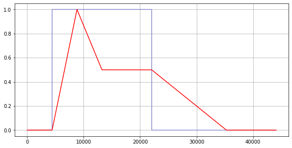
The Jupylet envelope generator expects a gate signal in its input to control the timing of the attack and release stages. Let’s see an example:
gate = LatencyGate()
adsr = Envelope(attack=0.1, decay=0.1, sustain=0.5, release=0.3)

gate.open(dt=0.1)
gate.close(dt=0.4)

g0 = gate(frames=44100)
e0 = adsr(g0)
Here is a plot of the generated envelope signal in red overlayed on top of the gate signal in light blue. Note how the gate signal correponds to the attack and release stages of the envelope:
And now that we know how to generate an evelope, let’s see how to apply it to our simple synthesizer:
class SimpleFMSynth3(GatedSound):

    def __init__(self):

        super().__init__()

        self.adsr = Envelope(attack=0.1, decay=0.1, sustain=0.5, release=0.5)

        self.osc0 = Oscillator('sine', 10)
        self.osc1 = Oscillator('sine')

    def forward(self):

        g0 = self.gate()
        e0 = self.adsr(g0)

        a0 = self.osc0() * 12
        a1 = self.osc1(a0, freq=self.freq)

        return a1 * e0
synth = SimpleFMSynth3()

synth.play(C6, 1/2)
await sleep(1)

synth.play(D6, 1/2)
await sleep(1)

synth.play(E6, 1/2)
await sleep(1)
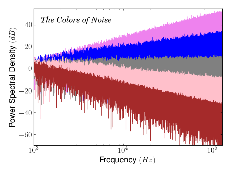
The Colors of Noise
I always thought the term white noise was just a figure of speech, a slang. I was wrong. It turns out the term white noise is so called in analogy to white light - that is, the signal you would get if you mix together all the different sine waves in the world, all equally powerful.
And just as it is with light, acoustic noise can have colors too, ranging from red noise where the low frequency waves are more powerful, to pink noise, to white noise where all frequencies have equal power, to blue noise, and finally to violet noise the high frequency waves are more powerful.
Imagine that we took apart a noise signal back to the separate sine waves it is made of and measured how powerful each of the sine waves is. If we did that we could then plot the power as a function of frequency, or as it is commonly known a power spectrum.
Since the power of all the sine waves that make up white noise is equal, the power spectrum of white noise would look like an horizontal line. Similarly the power spectrum of red and pink noise would look like a downward slope and that of blue and violet noise would look like an upward slope, as illustrated in the following figure (from Wikimedia Common):
You can create a noise generator by specifying its color name or a value between -6 for red noise, and 6 for violet noise. Let’s create and play some violet noise:
noise = Noise('violet')
sd.play(noise(frames=44100))
Noise generators can be used to create a variety of effects. One interesting application is to use red noise to modulate the frequency of another signal:
class Wobbly(GatedSound):

    def __init__(self):

        super().__init__()

        self.adsr = Envelope(attack=0.01, decay=0.5, sustain=0., release=0., linear=False)

        self.noise = Noise('red')
        self.osc0 = Oscillator('tri')

    def forward(self):

        g0 = self.gate()
        e0 = self.adsr(g0)

        n0 = self.noise()
        a0 = self.osc0(n0, freq=self.freq)

        return a0 * e0


wobbly = Wobbly()

wobbly.play_poly(C5)
await sleep(1/4)

wobbly.play_poly(E5)
await sleep(1/4)

wobbly.play_poly(G5)
await sleep(1/4)

wobbly.play_poly(B5)
await sleep(1/4)

wobbly.play_poly(C6)
await sleep(1)
Filters
The next staple element of sound synthesis up our sleeve is the audio filter. Filters are used in subtractive synthesis to attenuate particular frequencies in an audio signal rich in harmonics, similar to how your lips attenuate the sound coming out of your mouth as you speak or sing.
Jupylet includes a resonant filter parameterized by a cutoff frequency, that can operate in one of three modes; as a lowpass filter that attenuates frequencies above the cutoff frequency, a highpass filter that attenuates frequencies below the cutoff frequency, or a bandpass filter that attenuates frequencies outside a band of frequencies centered around the cutoff frequency.
As we saw above, white noise is made of sine waves of all frequencies, all having equal power. We can therefore apply a filter to white noise to see how it attenuates the power of different frequencies; Let’s do that with a lowpass filter and a cutoff frequency of 3000Hz:
noise = Noise('white')
lowpass = ResonantFilter(3000, 'lowpass')

n0 = noise(frames=44100 * 128)
a0 = lowpass(n0)

get_power_spectrum_plot(a0, xlim=(0, 8000), ylim=(20, 70))
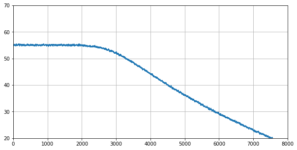
What a beauty. Now let’s try it again with some resonance at the cutoff frequency:
noise = Noise('white')
lowpass = ResonantFilter(3000, 'lowpass', resonance=2)

n0 = noise(frames=44100 * 128)
a0 = lowpass(n0)

get_power_spectrum_plot(a0, xlim=(0, 8000), ylim=(20, 70))
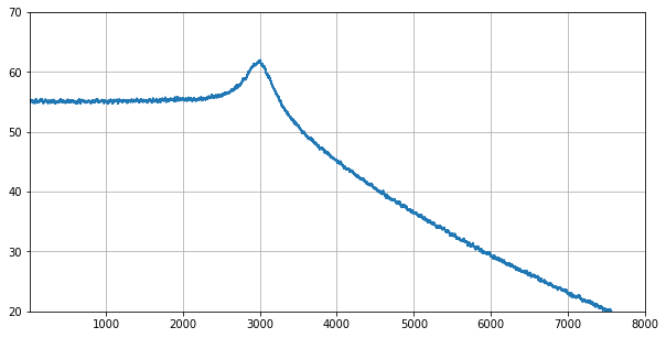
A resonant filter amplifies the frequencies around its cutoff frequency. It works similar to the resonance chamber of a guitar in that it is designed to amplify particular frequencies.
You may have wondered about the little waves that were visible in the antialiased sawtooth wave that we saw in the beginning of this chapter. They were there because a sawtooth wave is actually made of many simple sine waves of different frequencies and power.
These waves are also called tones or partials. The preceived pitch of the sawtooth wave is determined by the partial with the lowest frequency, which is called the fundamental. In a sawtooth wave, the frequencies of all the partials are interger multiples (also called harmonics) of the fundamental frequency, and their amplitude is inversely proportional to the integer multiple.
You can read more about it in the Wikipedia article on the Harmonic series.
OK, it’s time to put it all together into a synthesizer inspired by the sound of the Roland TB-303 Bass Line. The distinctive sound of the TB-303 is created by sweeping the cutoff frequency of a resonant lowpass filter from an initial high cutoff frequency down to the frequency of the note being played. To implement the sweep we employ a second envelope and configure it to decay nonlinearly from 1 to 0, and then we use it to modulate the cutoff frequency of the filter. As usual the modulation is done in logarithmic scale with semitones as units.
class TB303(GatedSound):

    def __init__(self):

        super().__init__()

        self.shape = 'sawtooth'
        self.resonance = 2
        self.cutoff = 0
        self.decay = 1

        self.env0 = Envelope(0.01, 0., 1., 0.01)
        self.env1 = Envelope(0., 1., 0., 0., linear=False)

        self.osc0 = Oscillator('sawtooth')

        self.filter = ResonantFilter(btype='lowpass', resonance=2)

    def forward(self):

        g0 = self.gate()

        e0 = self.env0(g0)
        e1 = self.env1(g0, decay=self.decay) * 12 * 8

        a0 = self.osc0(shape=self.shape, freq=self.freq)

        a1 = self.filter(
            a0,
            key_modulation=e1+self.cutoff,
            resonance=self.resonance,
            freq=self.freq,
        )

        return a1 * e0
Note
We declared the shape, resonance, cutoff, and decay variables as
members of the synthesizer class since this will enable us to specify
their values in calls to the use() and play() functions - for
example play(C4, 1/2, resonance=4, decay=2).
And now that the synthesizer is ready let’s instantiate it, set up a nice reverb effect, and start two simple simultaneous loops:
tb303 = TB303()

set_effects(ConvolutionReverb(impulse.InsidePiano))


@app.sonic_live_loop2
async def loop0():

    use(tb303, resonance=8, decay=1, cutoff=12, amp=1)

    play(C3, 1/2)
    await sleep(2)

    play(G2, 1/2)
    await sleep(2)

    play(Ds3, 1/2)
    await sleep(2)

    play(C3, 1/2)
    await sleep(2)


@app.sonic_live_loop2
async def loop1():

    use(tb303, resonance=8, decay=1/8, cutoff=48, amp=1)

    play(C2, 1/8)
    await sleep(1/4)

    play(C3, 1/8)
    await sleep(1/4)
Note
If you update a live loop decorated with @app.sonic_live_loop2
the new code will kick in once the current cycle through the loop
completes.
What Next?
Now it’s up to you. There are plenty of subjects we did not cover here but what has been covered should be just enough to get you started like a ballistic missile into sound synthesis play land.
Go on and create your own synthesizers and even your own components and algorithms; the main take away is that this framework gives you complete flexibility to create whatever you imagine; this is exactly how all the existing components and effects came to be.
One thing to keep in mind though, is that sound processing is real time, and you should therefore code your algorithms to be as efficient as possible.
Finally, the world of sound synthesis is as deep and as wide as an ocean and there is a tremendous amount of information online. However, if I need to pick one starting point to recommend it would be the online article series by Sound On Sound called Synth Secrets.