PROGRAMMING 3D GRAPHICS

Python in Space

Programming 2D games is awesome, but if you are anything like me what really blows your mind is 3D graphics; and yes, you can do it in Python!

Nevertheless, programming 3D games can be more demanding than programming 2D games. It involves using more complex tools, new concepts like lights and cameras, and some understanding of algebra in 3D space.

To help you get started I have created a 3D version of the spaceship game. You can find the notebook at examples/12-spaceship-3d.ipynb. Run it and open the magical portal to 3D space:

Blending in

In 2D game programming you may use a simple image editor to create game assets. The 3D parallel of the 2D image editor is a 3D modelling program. 3D modelling programs are complex tools and it takes time to master them. The great news is that one of the best tools around is completely free.

Blender is a free open source and totally awesome 3D creation suite, and Jupylet is designed to load assets created with it.

To get started with Blender I recommend the wonderful youtube videos by Grant Abbitt:

• Learn Blender 3 for Complete Beginners

• Beginner Exercises

• Sculpting

• Unwrapping & Placing 2d Textures

You may recognize the lego bricks in the lego notebook at examples/13-lego-3d.ipynb. They were created by following Abbitt’s beginner exercises.

How to export a Blender scene:

Jupylet can load Blender scenes exported using the glTF 2.0 format. To properly export a scene in this format follow these steps:

• Apply scale to all scene objects - to apply scale to an object select it and press CTRL+A.

• Choose export scene as glTF 2.0 format from the File menu.

• In the Format option select glTF Separate mode.

• Select the option to include the Cameras and Punctual Lights.

• Select the transform option named +Y Up.

• Select the option to Apply Modifiers

• Select the options to include UVs, Normals, and Materials.

• Set the file name and export.

The export should create a .gltf file, a .bin file, and image files for all the textures in the scene.

Note

• At the moment Jupylet does not load animations.

• Jupylet can load directional lights, spot lights, and point lights. However, at the moment point lights will only cast shadows in a 90 degrees cone. To properly set the cone’s direction, temporarily change the point light to spot light, set its direction and then switch it back to point light.

Lights, Camera, Action!

Modern API for 3D graphics are very flexible and may possibly accomodate any visual idea you may have regardless of how wild it may be.

However, when many people think of 3D graphics we often imagine being able to move around in an environment that is reminiscent of real life in some ways; most notably the role played by light and the way it interacts with objects in the environment, affecting their color and casting their shadow.

To make this possible, 3D game engines and 3D creation software such as Blender employ concepts we are familiar with from real life such as scenes, lights, cameras, and materials.

When you load an exported Blender scene into Jupylet, it is represented as a collection of lights, cameras, meshes (i.e. scene objects), and materials.

You can access, introspect, and manipulate these objects, to bring the scene to life. Let’s see how it is done in examples/12-spaceship-3d.ipynb.

We start by loading the exported Blender scene:

from jupylet.loader import load_blender_gltf

scene = load_blender_gltf('./scenes/moon/alien-moon.gltf')

Shadows are turned off by default. You can turn them on with:

scene.shadows = True

If you just want to draw the scene, simply call the scene.draw() method in the render() function. That’s it:

@app.event
def render(ct, dt):

    app.window.clear()
    scene.draw()

The best way to get a grasp on these concepts is to play around with the various objects in the scene. Let’s modify the camera’s field of view:

camera = scene.cameras['Camera']

camera.yfov = 0.4

If the game is running you should see the camera zoom in. If you increase the field of view the camera would appear to zoom out.

Note

In Jupyter you can manipulate the properties of objects while the game is running and see the effect immediately and interactively.

Let’s turn the color of the sun into bright red:

sun = scene.lights['Light.Sun']

sun.intensity = 16
sun.color = 'red'

Let’s make the moon twice as big:

moon = scene.meshes['Moon']

moon.scale *= 2

Take a few minutes to play around with the objects of the scene and you will soon get the idea. After all it’s not rocket science.

Note

In Jupyter you can find out the various method and properties of an object with the auto complete function. e.g. type moon. (don’t forget the dot) and then tap the Tab key.

A Little Bit of Math

Let’s move the alien one unit to the right:

alien = scene.meshes['Alien']

alien.position.x += 1

You should be able to notice it moved a little to the right.

Note

We are not specifying coordinates using pixels any more since we are not moving the alien on screen but in 3D space.

Now let’s move it one and a half units up:

alien.position.y += 1.5

So far nothing surprising. Now let’s try something new and move it 2 units towards us:

alien.position.z += 2

Coordinates in 3D space have 3 components x, y, z, with the z axis pointing towards us as shown in this figure:

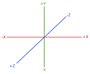
More generally the (x, y, z) components combined are called a vector:

In []: alien.position
Out[]: vec3( 1, 1.5, 2 )

Note

The In []: and Out []: notation in the example above is used in Jupyter notebooks to help us distinguish between what we type in and what Python prints out in response.

Jupylet uses a wonderful Python module called PyGLM for vector math. It is super fast and very convenient. Check it out!

Let’s define an arbitrary displacement in space and use it to move our alien:

import glm

displacement = glm.vec3(0.2, 1, 0.33)
alien.position += displacement

Are you ready for your first 3D animation? Type and run the following code in the spaceship 3D notebook while the game is running:

import asyncio

for i in range(100):
    alien.position += displacement / 30
    await asyncio.sleep(1/30)

If you did it correctly, you should see the alien drift away in the direction of the displacement we defined above.

If you know a little bit of Python you may be wondering why we have used the strange looking await asyncio.sleep(1/30) instead of the standard time.sleep(1/30). The simplistic answer is that the asyncio.sleep function is special in that it tells Python it can go do other stuff until the sleep period is over, where other stuff includes important other stuff like carrying on with all the other gazillion computations required for keeping the game going.

However, while the screen kept updating and the alien kept spinning as it drifted away, you may have noticed that the game does not seem to respond to key presses while the animation is running and that you therefore cannot navigate the spaceship (with the W, A, and D keys).

The explanation for why this is happening is complicated and involves advanced Python, but the good news is that we can easily fix it. Run the following code in the game notebook and the alien should start drifting indefinitely and this time you should be able to chase it by navigating the ship:

velocity = glm.vec3(0.2, 1, 0.33)

@app.run_me_every(1/30)
def drift(ct, dt):
    alien.position += velocity * dt

Notice how we changed the vector name from displacement to velocity and now we suddenly have a proper physics equation driving our little animation (ds = v * dt).

Type the following to bring back the alien to its original position:

alien.position = glm.vec3(0)

Or stop the alien in its tracks with:

app.stop(drift)

Our alien has two interesting vector attributes alien.up and alien.front. The up vector can be visualized as a personal +y axis that always points upward through the alien’s head regardless of the alien’s orientation, while the front vector always points in the direction the alien is facing.

The spaceship notebook includes a spin() function that keeps the alien spinning clockwise perpetually. Let’s combine this spinning with a small displacement in the direction of the up vector to make the alien swim through space in circles:

@app.run_me_every(1/30)
def swim(ct, dt):
    alien.position += alien.up * dt

More generally these personal up and front vectors are known as the local coordinate system of the alien; i.e. a personal set of +x, +y, +z axes that rotate along with the alien’s orientation.

Here is a version of the swim() function that uses the local coordinate system explicitly:

y_direction = glm.vec3(0, 1, 0)

@app.run_me_every(1/30)
def swim(ct, dt):
    alien.move_local(y_direction * dt)

Finally we arrive at the trickiest of all functions - rotation in 3D space. The default spin() function actually performs a clockwise roll rotation; that is, a clockwise rotation around the front (+z) axis. Let’s replace it with a proper ballet dancing spinning around the up (+y) axis:

import math

@app.run_me_every(1/30)
def spin(ct, dt):
    alien.rotate_local(2 * math.pi * dt, y_direction)

The alien.rotate_local(angle, axis) function expects two arguments; an angle specifying how many radians to rotate, and a vector specifying the axis to rotate around.

By multiplying 2 * math.pi, the number of radians in a full circle, by dt, the number of seconds since the last time the function was called, we make the alien spin at the rate of one full rotation per second (think about it).

The Sky in a Box

You may be surprised to learn that the beautiful nebula laden sky of the spaceship demo is implemented as six carefully prepared images texturing the six faces of a virtual cube positioned around the game camera such that the viewer is always at the center of the cube.

Technically it is a form of anamorphosis that requires the viewer to occupy the exact middle of the cube in order to enjoy the optical illusion, just as 3D street art and drawings require the viewer to observe them from a particular vantage point.

Here is an illustration of the nebula skybox images laid out as the unwrapped faces of the skybox cube (i.e. its left, front, right, back, top, and bottom faces):

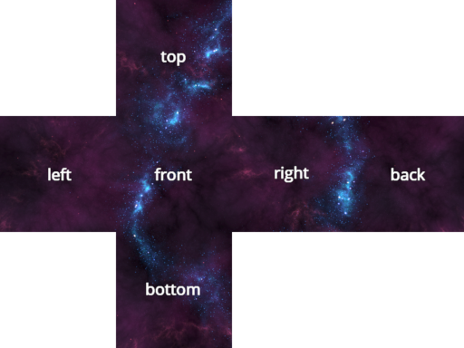
In 3D gaming skyboxes can be used to create a powerful atmospheric effect and to give a sense of depth to an environment.

The nebula skybox used in the spaceship game was created by Spacescape and you can find many other skyboxes and tools and guides for creating them online.

Back to the spaceship notebook, the nebula skybox is loaded with the following statement:

from jupylet.model import Skybox

scene.skybox = Skybox('./scenes/moon/nebula/nebula*.png', intensity=2., flip_left_right=True)

The first argument to the Skybox constructor is a glob path pattern that matches the six skybox images. The intensity argument adjusts the exposure of the images (we brighten them a little to make the effect more pleasing). Finally, try toggling the flip_left_right argument if your skybox appears to be badly stiched.

Diving into OpenGL

Over the years many sophisticated algorithms have been developed to enable computer graphics to reproduce the visual effect of the interaction of light and matter. By default Jupylet employs some of these algorithms to approximate the way Blender would render a 3D scene.

However, you are not limited in any way to the default Jupylet renderer. Jupylet is built on top of the wonderful ModernGL library, which is an efficient wrapper around the OpenGL API. By using ModernGL and the OpenGL API you are free to program your own GPU shaders and create any visual effect you want, from cartoon like shading to mesmerizing music visualizations (see Shadertoys below), to any effect you are imaginative enough to dream up and skilled enough to program.

If you would like to dive into OpenGL and shading check out learnopengl.com.

Shadertoys

Once you get a little comfortable with OpenGL and the GLSL shader programming language, Shadertoys are a great way to practice and upgrade your skills by programming and sharing fragment shaders online:

Two online tutorials worth checking out are The principles of painting with maths and the series ShaderToy Tutorials.

You can render shadertoys in Jupylet with the Shadertoy class. For example here is how to create and render the default shadertoy.com shader:

from jupylet.shadertoy import Shadertoy

st = Shadertoy("""

    void mainImage( out vec4 fragColor, in vec2 fragCoord )
    {
        // Normalized pixel coordinates (from 0 to 1)
        vec2 uv = fragCoord/iResolution.xy;

        // Time varying pixel color
        vec3 col = 0.5 + 0.5*cos(iTime+uv.xyx+vec3(0,2,4));

        // Output to screen
        fragColor = vec4(col,1.0);
    }

""")

@app.event
def render(ct, dt):

    app.window.clear()
    st.draw()

You can set the input of any of the 4 channels of a shadertoy with the Shadertoy.set_channel() method. For example to set a texture to channel 0:

st.set_channel(0, 'images/alien.png')

You can also set the input with an audio signal as a Numpy array. Shadertoy expects the signal as an array of 2 rows, 512 samples, and two channels (left, right) with values between 0 and 255. The first row should be the power spectrum of the signal and the second row should be amplitude samples of the signal. You can use the convenience function get_shadertoy_audio() to prepare the required input from the audio system output. For example:

from jupylet.shadertoy import get_shadertoy_audio

st.set_channel(0, *get_shadertoy_audio())

Finally, you can chain shaders by setting one shader as the input of another and even create cycles to produce interesting effects. For a basic example of displaying a shadertoy see the examples/16-shadertoy-demo.ipynb notebook. For a more advanced example see the audio visualization shader by Alban Fichet in the examples/14-piano.ipynb notebook.